The Back-And-Forth Method (BFM) for Wasserstein Gradient Flows¶

This page provides documentation for the source code used in the paper The back-and-forth method for Wasserstein gradient flows [1]. A MATLAB wrapper to our C++ code is provided here: https://github.com/wonjunee/wgfBFMcodes.

Introduction¶

We are interested in simulating Darcy’s law (also known as the generalized porous medium equation)

\[\begin{split}\partial_t \rho - \nabla \cdot (\rho \nabla \phi) = 0\\ \phi = \delta U(\rho)\end{split}\]

on a domain $\Omega\subset\mathbb{R}^2$. This equation describes the evolution of a mass density $\rho$ flowing along a pressure gradient $\nabla \phi$ generated by an energy functional $U$. The evolution of the density can be approximated by a discrete-in-time scheme known as the JKO scheme [3]. Given an initial density $\rho^{(0)}$, this scheme constructs approximate solutions by iterating

(1)¶\[\rho^{(n+1)} := \underset{\rho}{\text{argmin}} \,\, U(\rho) + \frac{1}{2\tau} W_2 (\rho, \rho^{(n)})^2.\]

Here, $\tau$ plays the role of a time step and $W_2(\cdot,\cdot)$ is the 2-Wasserstein distance. We extend the back-and-forth method (BFM) [2] for optimal transport to efficiently solve (1). The BFM solves (1) via the dual formulation

(2)¶\[\sup_{\phi,\psi} \int_\Omega \psi(x) \,\rho^{(n)}(x) dx - U^*(\phi),\]

where the supremum runs over functions $\phi,\psi\colon \Omega \rightarrow \mathbb{R}$ satisfying

\[\psi(x) - \phi(y) \leq \frac{|x-y|^2}{2\tau}.\]

Installation¶

Requirements: FFTW (download here), MATLAB.

Clone or download the repository:

git clone https://github.com/wonjunee/wgfBFMcodes
cd wgfBFMcodes/

Compile: in a MATLAB session run

mex -O CFLAGS="\$CFLAGS -std=c++11" src/wgfslow.cpp -lfftw3
mex -O CFLAGS="\$CFLAGS -std=c++11" src/wgfinc.cpp -lfftw3

This will produce two MEX functions that you can use in MATLAB: wgfslow for slow diffusions and wgfinc for incompressible energies.

You may need to use -I and -L to link to the FFTW3 library, e.g. mex -O CFLAGS="\$CFLAGS -std=c++11" src/wgfslow.cpp -lfftw3 -I/usr/local/include. See this page for more information on how to compile MEX files.

Slow diffusion¶

Usage¶

In a MATLAB session, the command

rhoFinal = wgfslow(rhoInitial, V, obstacle, m, gamma, ...
        maxIters, TOL, tau, nt, folder, verbose);

computes the JKO iterates $\rho^{(n)}$ from an initial density $\rho^{(0)}$ with the internal energy

(3)¶\[U(\rho) = \frac{\gamma}{m-1} \int_\Omega \rho^m(x) dx + \int_\Omega V(x)\,\rho(x)dx.\]

The iterates $\rho^{(n)}$ will be stored as binary files rho-0000.dat, rho-0001.dat, etc in a user-specified folder.

Input:

rhoInitial : The nonnegative initial density $\rho^{(0)}$.
V : The potential function $V(x)$.
obstacle : An obstacle in $\Omega$. Any positive values indicate the obstacle. The densities $\rho^{(n)}$ will always be $0$ on the obstacle.
m : The constant $m$ in the internal energy $U$.
gamma : The constant $\gamma$ in the internal energy $U$.
maxIters : The maximum number of inner loop iterations $k$ of the BFM in each outer iteration of the JKO scheme.
TOL : The tolerance for the BFM. Once the error $\| T_{\phi_k\#} \rho^{(n)} - \delta U^*(\phi_k) \|_{L^1}$ becomes less than the tolerance, the algorithm stops the BFM and proceeds to the next outer iteration $n+1$.
tau : The time step $\tau$ in (1).
nt : The number of outer iterations $n$ of the JKO scheme.
folder : Path to the folder where the successive iterates $\rho^{(n)}$ will be saved. Don’t include a trailing slash.
verbose : 1 - print out process in c++ code. 0 - be silent.

Output:

rhoFinal : The final density $\rho^{(nt)}$ after nt outer iterations.

Example¶

We compute the Wasserstein gradient flow of a slow diffusion energy (3) on the 2d domain $[0,1]^2$.

We discretize the problem on a $512\times 512$ grid and plot the densities.

% Parameters
n = 512;             % The size of the n x n grid
maxIters = 200;      % Maximum number of BFM iterations
TOL = 1e-2;          % Tolerance for BFM
nt  = 60;            % Number of outer iterations
tau = 0.005;         % Time step in the JKO scheme
m   = 2;             % m in the internal energy
gamma = 0.05;        % gamma in the internal energy
folder = 'data';     % Output directory
verbose  = 1;        % pPrint out logs


[x,y] = meshgrid(linspace(0,1,n));

% Initial density
rhoInitial = zeros(n);
idx = (x-0.5).^2 + (y-0.5).^2 < 0.1^2;
rhoInitial(idx) = 1;
rhoInitial = rhoInitial / sum(rhoInitial(:)) * n^2;

% Potential
V = sin(3*pi*x) .* sin(3*pi*y);

% No obstacle
obstacle = zeros(n);

% Plots
subplot(1,2,1)
contourf(x, y, rhoInitial)
title('Initial density')
axis square

subplot(1,2,2)
contourf(x, y, V);
title('Potential V')
axis square

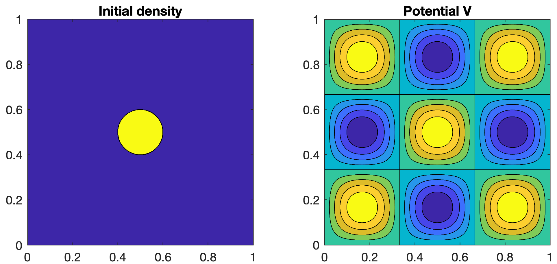
Here $\rho^{(0)}$ is renormalized so that $\int_\Omega\rho^{(0)}(x)dx=1$. Now run the algorithm

rhoFinal = wgfslow(rhoInitial, V, obstacle, m, gamma, ...
        maxIters, TOL, nt, tau, folder, verbose);

Output:

XXX Slow Diffusion XXX

n    : 512
nt   : 60
tau  : 0.005
m    : 2
gamma: 0.05
Max Iteration : 200
Tolerance     : 0.01

CPU time for FFT: 0.005817 seconds.

The total mass : 1
Iter : 1
50      Dual value: 1.2282      L1 error: 0.0262
100     Dual value: 1.2280      L1 error: 0.0193
150     Dual value: 1.2279      L1 error: 0.0172

...

Iter : 60
1       Dual value: -0.2241     L1 error: 0.0024

CPU time for GF: 70.906929 seconds.

Make movie

fig = figure;
movieName = 'movie.gif';

for i = 0:nt
    file = fopen(sprintf("%s/rho-%04d.dat", folder, i), 'r');
    rho = fread(file, [n n], 'double');
    imagesc(rho)
    axis xy square
    set(gca,'XTickLabel',[], 'YTickLabel',[])

    frame = getframe(fig);
    im = frame2im(frame);
    [X,cmap] = rgb2ind(im, 256);

    % Write to the GIF file
    if i == 0
        imwrite(X, cmap, movieName, 'gif', 'Loopcount',inf, 'DelayTime',0.03);
    else
        imwrite(X, cmap, movieName, 'gif', 'WriteMode','append', 'DelayTime',0.03);
    end
end

The file movie.gif

Incompressible energy¶

Usage¶

In a MATLAB session, the command

rhoFinal = wgfinc(rhoInitial, V, obstacle, maxIters, TOL, ...
        tau, nt, folder, verbose);

computes the JKO iterates $\rho^{(n)}$ from an initial density $\rho^{(0)}$ with the internal energy

(4)¶\[U(\rho) = \int_\Omega u_\infty(\rho(x)) dx + \int_\Omega V(x)\,\rho(x)dx.\]

Here $u_\infty(\rho)=0$ if $0\le\rho\le 1$ and $+\infty$ otherwise.

The iterates $\rho^{(n)}$ will be stored as binary files rho-0000.dat, rho-0001.dat, etc in a user-specified folder.

Input:

rhoInitial : The nonnegative initial density $\rho^{(0)}$.
V : The potential function $V(x)$.
obstacle : An obstacle in $\Omega$. Any positive values indicate the obstacle. The densities $\rho^{(n)}$ will always be $0$ on the obstacle.
maxIters : The maximum number of inner loop iterations $k$ of the BFM in each outer iteration of the JKO scheme.
TOL : The tolerance for the BFM. Once the error $\| T_{\phi_k\#} \rho^{(n)} - \delta U^*(\phi_k) \|_{L^1}$ becomes less than the tolerance, the algorithm stops the BFM and proceeds to the next outer iteration $n+1$.
tau : The time step $\tau$ in (1).
nt : The number of outer iterations $n$ of the JKO scheme.
folder : Path to the folder where the successive iterates $\rho^{(n)}$ will be saved. Don’t include a trailing slash.
verbose : 1 - print out process in C++ code. 0 - be silent.

Output:

rhoFinal : The final density $\rho^{(nt)}$ after nt outer iterations.

Example¶

We compute the Wasserstein gradient flow of an incompressible energy (4) on the 2d domain $[0,1]^2$.

We discretize the problem on a $512\times 512$ grid and plot the densities.

n = 512;             % The size of the n x n grid
maxIters = 300;      % Maximum number of BFM iterations
TOL = 3e-2;          % Tolerance for BFM
nt  = 180;           % Number of outer iterations
tau = 0.005;         % Time step in the JKO scheme
folder = 'data';     % Output directory
verbose  = 1;        % Print out logs


[x,y] = meshgrid(linspace(0,1,n));

% Initial density
rhoInitial = zeros(n);
idx = (x-0.25).^2 + (y-0.75).^2 < 0.15^2;
rhoInitial(idx) = 1;

% Potential
V = 3 * ((x-0.7).^2 + (y-0.3).^2);

% Add an obstacle
obstacle = zeros(n);
idx = (x-0.5).^2 + (y-0.5).^2 < 0.1^2;
obstacle(idx) = 1;

% Plots
subplot(1,3,1)
contourf(x, y, rhoInitial)
title('Initial density')
axis('square')

subplot(1,3,2)
contourf(x, y, V);
title('Potential V')
axis('square')

subplot(1,3,3)
contourf(x, y, obstacle)
colormap(gca, 'copper')
title('Obstacle')
axis('square')

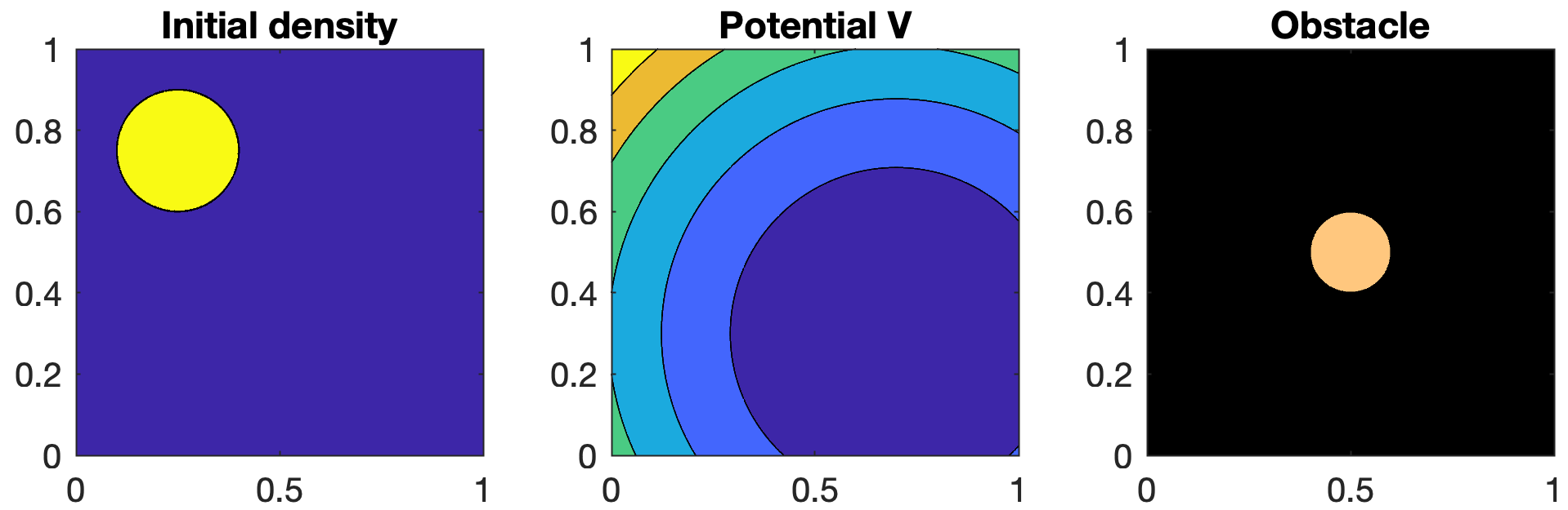
Run the algorithm

rhoFinal = wgfinc(rhoInitial, V, obstacle, maxIters, TOL, nt, tau, ...
        folder, verbose);

Output:

XXX Incompressible Flow XXX

n    : 512
nt   : 180
tau  : 0.005
Max Iteration : 300
Tolerance     : 0.03

CPU time for FFT: 0.295334 seconds.

Total mass : 0.0703964
Iter : 1
10      dual value: 0.085350    L1 error: 0.1135
20      dual value: 0.085378    L1 error: 0.0807
30      dual value: 0.085386    L1 error: 0.0628
40      dual value: 0.085390    L1 error: 0.0525
50      dual value: 0.085391    L1 error: 0.0446
56      dual value: 0.085392    L1 error: 0.0407

...

Iter : 180
7       dual value: 0.002379    L1 error: 0.0329

CPU time for GF: 616.0 seconds.

Note that here there is a ceiling contraint $\rho(x)\le 1$ so the total mass must be less than 1. Make movie

fig = figure;
movieName = 'movie.gif';

for i = 0:nt
    file = fopen(sprintf("%s/rho-%04d.dat", folder, i), 'r');
    rho = fread(file, [n n], 'double');
    imagesc(rho)
    axis xy square
    set(gca,'XTickLabel',[], 'YTickLabel',[])

    frame = getframe(fig);
    im = frame2im(frame);
    [X,cmap] = rgb2ind(im, 256);

    % Write to the GIF file
    if i == 0
        imwrite(X, cmap, movieName, 'gif', 'Loopcount',inf, 'DelayTime',0.001);
    else
        imwrite(X, cmap, movieName, 'gif', 'WriteMode','append', 'DelayTime',0.001);
    end
end

The file movie.gif

References¶

[1] Matt Jacobs, Wonjun Lee, and Flavien Léger. The back-and-forth method for Wasserstein gradient flows. Submitted. 2020.

[2] Matt Jacobs and Flavien Léger. A fast approach to optimal transport: the back-and-forth method. Numerische Mathematik (2020): 1-32.

[3] Richard Jordan, David Kinderlehrer, and Felix Otto. The variational formulation of the Fokker–Planck equation. SIAM journal on mathematical analysis (1998): 29(1), 1–17.

Table of Contents

Navigation

The Back-And-Forth Method (BFM) for Wasserstein Gradient Flows¶

Introduction¶

Installation¶

Slow diffusion¶

Usage¶

Example¶

Incompressible energy¶

Usage¶

Example¶

More Videos¶

References¶